
The material presented in this tutorial is based primarily on the material given in the 'Tutorial Manual' of the SYBYL software package.
After this tutorial you will be able to, a.o.:
BUILD/EDIT >>> ZAP (DELETE) MOLECULE
Use the RESET gadget to reset EVERYTHING
VIEW >>> DELETE ALL BACKGROUNDS
From the FILE >>> READ... menu,
Alternatively, you may use your own sketch model of atropine.
In that case, choose the name from the 'Files' box.
Do make sure 'atropine' is read into workarea M1.
COMPUTE >>> MINIMIZE...
Fig.8 Energy dialog box
Press Minimize Details... button.
Fig.9 Minimization details dialog box
Type atropine_1 as the job name in Minimize dialog box.
Fig.10 Minimize dialog box after changes
Press OK.
The minimization has now been submitted to run in batch mode. Proceed to the next step of
this tutorial while this batch job is executing.
VIEW >>> LABEL >>> ATOM ID...
Note that during the selection of atoms to be labeled, the atoms are
highlighted.
Press END on the Atom selector box
BUILD/EDIT >>> MODIFY >>> TORSION...
COMPUTE >>> MINIMIZE...
The minimization of the modified model has now been submitted to run in
batchmode also.
Finishing batch jobs signal to the user by messages such as:
INFO: NetBatch job atropine_1 completed on machine cammsg1.
INFO: Wed May 29 11:31:22 MDT 1996
When both optimizations are done, i.e. the above message has appeared
for both atropine_1 and atropine_2, you can continue
comparing the results. Meanwhile, you could exercise rotating, scaling,
and labeling the model or check the geometry using ANALYZE >>>
MEASURE... and selecting one of the options presented.
Make sure all labels are turned off. (VIEW >>> UNLABEL...
etc.)
Read the results of both optimizations into workareas M2 and M3:
FILE >>> READ...
(Alternatively, if you have not been able to optimize both raw models of
atropine, you can READ them from the ta_demo: directory as
atropine_1.mol2 and atropine_2.mol2.)
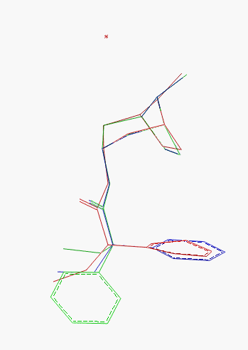
Three structures are now displayed. Try superimpose the models manually
using the ringsystem of the raw model as reference point. Use the Work Area
gadget to toggle the Display Area to be rotated from G to
D1, D2, D3 and D4 and back to G.
BUILD/EDIT >>> ZAP (DELETE) MOLECULE.
FILE >>> READ...
Undisplay all H atoms using either the command line:
or the equivalent from the menu (VIEW >>> UNDISPLAY >>> M2 >>> ATOM TYPE >>>
H and pressing OK. Likewise for work area M3).
ANALYZE >>> FIT ATOMS...
Repeat this sequence for the models in work areas M1 and M3, using M1
again as reference.
Change the display back to FULL from the Display Options
menu, and try to color the molecules differently using VIEW >>> COLOR >>>
ATOMS... and selecting all atoms from one work area and assign a
specific color to the selected set.
Fig.11 Final display
Compare the potential energies of the two optimized models using:
COMPUTE >>> ENERGY... Note that the energy is written to the text window.
This concludes the minimizing small molecule tutorial.
We suggest that you repeat this tutorial on your own molecules of interest.
Other SYBYL tutorials:
Return to the
main SYBYL tutorial page.
Clearing work areas
If there is more than one molecule on the screen, click ALL, then
OK to wipe them all.
Use the DISPLAY OPTIONS to reset to FULL screen mode.
Read molecule 'atropine'
type ta_demo:atropine_raw.mol2
in the 'File to read' area. (Press OK)Setting up and submitting the minimization
Press the MODIFY... button.
Set the appropriate options to make the Energy dialog box looks
like the one in Fig.8. In particular:
- Select TRIPOS in the Force Field option menu,
- Select GASTEIGER-HUCKEL in the Charges option menu.
Press OK.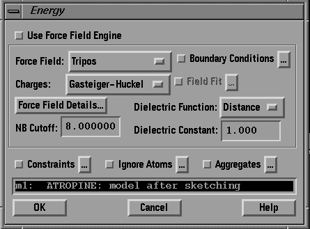
Make the appropriate selections so that the dialog box matches the one
show in fig.9. In particular:
- Increase the maximum number of iterations to 1000.
- Decrease the Non-bonded reset to 5.
- Decrease the gradient threshold to 0.005.
- Set the color option to Force.
Press OK.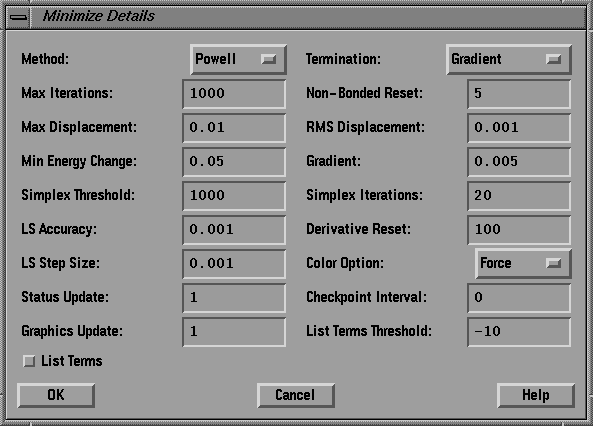
Select the SHORT 'machine' where the calculation is to be run.
Check the RUN IN BATCH box. The dialog box should look like the one
in fig.10.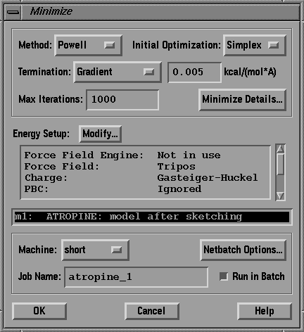
Optimizing a modified atropine model
While the optimization of the sketched model of atropine is proceeding
in batch mode, the raw model is slightly changed to adopt a different
conformation. The modified model is optimized also, and the two
conformations are compared visually.
Select ALL and change the logical operator UNION into
DIFFERENCE
Select ATOM TYPES... and toggle H on (Press OK to
leave the Atom type selector box).
Select atoms 9, 10, 11 and 12 subsequently,
and note that the current torsion is written to the text area (180 degrees).
Move the mouse into the Torsion angle value box and enter -60
(Press OK).
Type atropine_2 as the job name in the Minimize dialog
box.
Leave all other options unchanged.
Press OK.Results
Use the RESET gadget to reset EVERYTHING.
Use the Display Options gadget:  , to set the
screen in quartered mode.
, to set the
screen in quartered mode.
In the Read File menu, change the File Type ALL button into
MOLECULE.
Select atropine_1.mol2 and make sure m2: <empty> is
highlighted. Press OK.
FILE >>> READ...
Select atropine_2.mol2 and make sure m3: <empty> is
highlighted. Press OK.
Select M1, the raw model (Press OK).
and type ta_demo:atropine_cry.mol2
in the 'File to read' area. (Press OK).
undisplay m2(<h>)
undisplay m3(<h>)
Activate the ADD.. button and then select matching atom pairs
from workareas M1 and M2 respectively.
Choose only the ring atoms.
Choose atoms from M1 first and then atoms from M2, making sure that the model
in workarea M1 is used as reference.
Select END from the atom selector box, when all pairs (8) are
selected.
Select SOLVE from the Fit Atoms menu and notice the model
in work area M2 changing its orientation.
and activating M2 (and later M3) and press
COMPUTE.